Fractal Architect 4 Help Index

Applies to:FA 4
So each iteration the renderer does this to the pool of point values:
(The triangle in the editor shows the affect of applying the matrix to a simple triangle. When you edit the triangle, you are in fact editing the transformation matrix.)
These output point values are added together to create the final output point values from the variation list calculations.
Apophysis introduced the concept of Pre, Normal, and Post variations.
The renderer, in applying variation calculations, will first calculate all the pre-variations, then the normal-variations, then the post-variations.
The output from a pre-variation becomes the input to normal variation. The summed output from the set of normal variations is the input to a post-variation.
So it effectively does this:
pre–1 ==> pre–2 ==> [ normal–1 + normal–2 + … ] ==> post–1 ==> post–2
Note the output from a pre becomes the input to either another pre or the input to all normal variations. Note the summed output from all normal variations becomes the input to the first post variation.
Pre_variations can be chained in series, so for pre_blur ==> pre_flatten
that means output points of pre_blur becomes the input points of the pre_flatten.
Post_variations can be chained in series too.
Normal variations are evaluated in parallel which means they can be evaluated in any order (because addition is cumulative and associative)
In Apophysis, the variation’s source code and specifically how that code handled the variation’s output values determined if a variation type would have pre, post, or normal behavior. (The community would add pre_ and post_ prefixes to the variation names too).
Thomas Ludwig noted that this behavior could be shifted to the renderer framework, so that any variation type could be used as a pre or post variation. His Chaotica renderer was the first renderer to implement this.
| Pre Variations | Normal variations | Post variations |
|---|---|---|
| inX ==> evaluate a new X | inX ==> evaluate a new X | outX ==> evaluate a new X |
| assign that new X to inX | add that X to outX | assign that new X to outX |
Pre_variations can be chained in series, so for pre_blur ==> pre_flatten that means input of one becomes the input of the next. Post_variations can be chained in series too. Normal variations are evaluated in parallel which means they can be evaluated in any order (because addition is cumulative and associative)
So: the renderer does this for a specific transform: evaluates pre_variations in series, then evaluates all normal variations in parallel, then evaluates post_variations in series. The order of evaluation for pre and post variations is determined by the ordering of those variation types in the variation set.
So think of this in another way. Variation calculations are just like electric current in a circuit. The flow (and order of execution) of calculations is like electric current in a circuit:
Pre and post variations are applied in series. The output from these variations become the input to the next step in the chain.
Normal variation calculations are applied in parallel. Summing the calculated results together is a parallel operation.
Fractal Architect extends this Apophysis innovation even further.
Think of the set of normal variations as a group, with the group’s output being the summation of the outputs from each variation in the group. These groups are called variation groups.
As with pre and post variations, the groups themselves can be linked in series. The output from one group becomes the input to the next group. The linked groups are called a Variation Group Chain
So it effectively does this (showing 3 variation groups in a chain here):
[ normal–1 + normal–2 + … ] ==> [ normal–1 + normal–2 + … ] ==> [ normal–1 + normal–2 + … ] OR
group–1 ==> group–2 ==> group–3
So with Fractal Architect, a flame fractal transform, no longer has a set of variations. It has instead a variation group chain, with each variation group being a set of variations. The case of a chain with just a single variation group, has the exact same rendering behavior as with Flam3/Apophysis.
Think of the Fractal Architect Variation Group Chain architecture as being a more general case. From the exact same group of variations as before, you get some completely new image creation capabilities.
If you open a normal Flam3 style fractal, you get a single Variation Group per transform. It can use pre and post variations that have been defined as part of the variation set. One limitation of this older architecture, is that you only get pre and post behavior from special variation types that are included in the variation set.
In the renderer, the evaluated output from a Variation Group becomes the input to the next Variation Group. So variation groups are evaluated in series. The order of evaluation inside a single variation group is the same as the old architecture.
So, that means Group#1 acts like a big Pre variation in affect to Group#2. Group#3 acts like a big Post variation in affect to Group#2. (Order of evaluation is: Group#1, then Group#2, then Group#3)
If we have Group #1 with a single transform instance julian#1 and Group#2 with a single transform instance linear#1, this has the same renderer output as we would get with a single Group having: pre_julian#1 and linear#1.
But there is no pre_julian variation type !! So using chained Variation groups, allows us to use normal variation types as pre/post variation types !
If you want traditional Flam3/Apophysis rendering behavior, just use a single variation group in each transform’s variation group chain. You will get identical renders with those traditional renderers.
So the step Apply Variation Calculations from above now becomes:
These output point values are added together to create the Group’s output point values
a) If there is a second variation group, take the first group’s output point values and use them as the input point values for the second variation group; calculate the 2nd group’s output point values.
b) If there are more groups in the chain, repeat the behavior of step a).
Take the last variation group’s output points and apply the post transformation matrix to them.
With the Variation Group Chain architecture, the need for specialized pre and post variation types is removed. Fractal Architect still fully supports traditional pre and post variation types. Older fractals that use them, will still render correctly.
With variation groups, the group ordering now determines pre and post behavior. The output from one group becomes the input to the next group.
Lets look at a set of traditional variations: - polar2 - pre_polar2 - post_polar2
So for a Apophysis transform with 2 variations in it: pre_polar2 and julian; Fractal Architect gives you 2 ways to get the same rendering behavior.
A) Single variation group with both pre_polar2 and julian.
[ pre_polar2 ==> julian ]
or
B) Two variation groups in a chain, each group has one variation
[ polar2 ] ==> [ julian ]
Note: we use polar2 – not pre_polar2 !!
Another change in Fractal Architect is that you can now have multiple instances of the same variation type in the same variation group. The app now appends the instance number everywhere you used to see
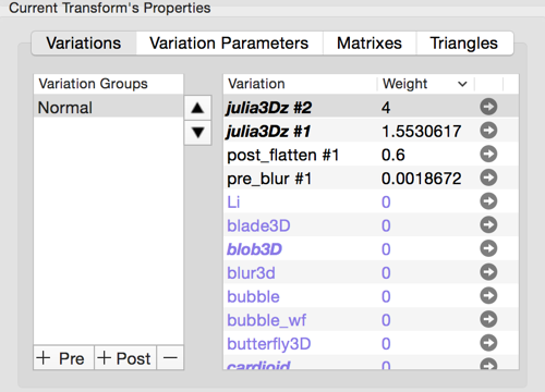
The Triangle Editor shows the Variation Group Chain and for the selected group it shows on top, the variations that have been chosen. The purple variation names are not instances, but are just a way to show the variation names which are available.
When you change a variation’s weight to non-zero, it becomes an instance. When you set a non-zero weight to zero, the variation instance is removed.
The bold variation names just show you as a reminder that that variation type has variation parameters for you to set as well.

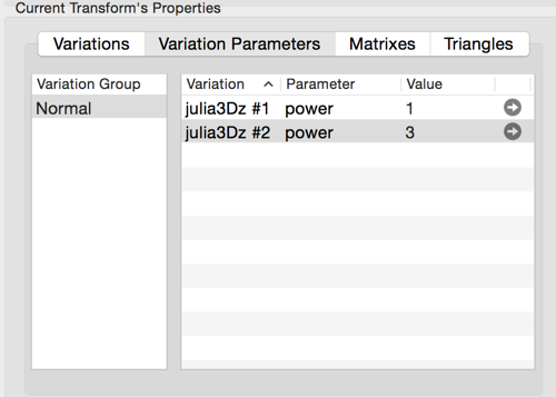
Variation parameters are instanced as well.

For the same fractal, here is a Fractal Info snippet showing a normal variation group and the same instanced variations.
Xform #2    weight: 0.1415  colorIndex: 0.9352  color_speed: 0.7964  opacity: 100% var_color: 1  rotates: YES
Variation Group Normal ========
    pre_blur #1: 0.0019
    julia3Dz #1: 1.5531  power: 1
    julia3Dz #2: 4  power: 3
    post_flatten #1: 0.6

    Pre:  1.0000000000  0.0000000000  0.0000000000
          0.0000000000  1.0000000000  0.0000000000
    Post: 1.0000000000  0.0000000000  0.0000000000
          0.0000000000  1.0000000000  0.0000000000
Instancing imposes a run-time overhead of doing variation calculations for each instance. So for the example shown, the julia3Dz calculations will be done twice, once per instance. In this example, the variation weights and the power parameter for the instances were different. This is effective use of instancing. The different power parameters between the instances cannot be simplified.
On the other hand, if both instances had the exact same parameter values, then the two instances could be merged into one instance (with its weight being the summation of the original instances’ weights).
Now lets use the example of two linear variation instances: linear#1 and linear#2.
Linear#1 has weight of 1 and linear#2 has weight 2.
Since the linear variation type has no variation parameters, you can get the same output with a single linear instance (using linear#1 with weight of 3). You can add the instances’ variation weights together and just use one instance with the summed weight.
That is more efficient as only one variation calculation is done instead of two.
Each xforms table has sub-tables holding all of the xform’s variation groups.
This snippet inserts a julia3D variation instance into
xform = flame.xforms[2]
table.insert(xform.variations, { name="julia3D",      weight=0.7, julia3D_power=-2 })
-- Randomly (33% probability) adds a Cpow variation to the Pre Variation Group for all xforms in the fractal
for i,v in ipairs(flame.xforms) do
    if math.random() < 0.3 then
        -- make sure there is a Pre Variation group to put the Cpow variation into
        if #v.preVarGroups == 0 then
            table.insert(v.preVarGroups, {})
        end

        table.insert(v.preVarGroups[1], { name="cpow", weight=math.random(),
                                            cpow_i = 0.5 + math.random() * 1.5,
                                            cpow_power = math.random(1, 5),
                                            cpow_r = 0.1 + math.random() * 2.9});
    end
end